Part 5: Data summarizing, reshaping, and wrangling with multiple tables
R Project files
Please download the part5 subfolder in this folder link Be sure to unzip if necessary. “Knit” the code/part5.Rmd file to install packages and make sure everything is working with data loading.
Class Video
View last year’s class and materials here.
Slides
During “Muddiest Parts” review, we will go over these slides
Another useful video
Dr. Kelly Bodwin’s Reshaping Data Video
For a short version, watch the pivot_longer excerpt about “working backwards” from a plot. Then watch the pivot_wider excerpt
Post-Class
Please fill out the following survey and we will discuss the results during the next lecture. All responses will be anonymous.
- Clearest Point: What was the most clear part of the lecture?
- Muddiest Point: What was the most unclear part of the lecture to you?
- Anything Else: Is there something you’d like me to know?
Muddiest Points
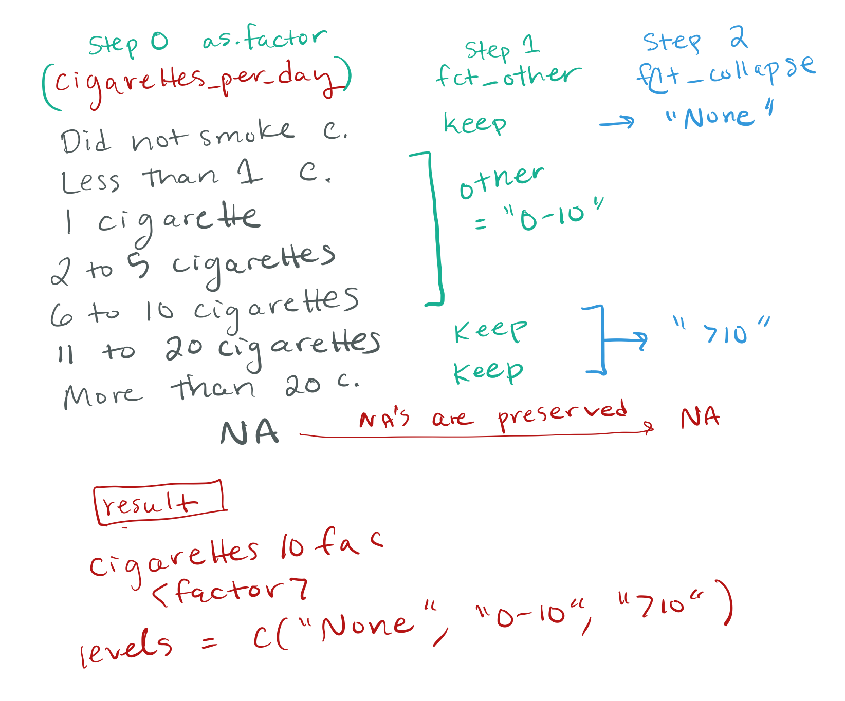
fct_other() and fct_collapse: I actually think I understand the point of each of these separately, but somehow using them together like in the example totally confused me. I’ll have to go look at it again later.
The data cleaning section where we used forcats since it was confusing as to how to use it.
when to use fct_collapse vs case when and when you would want to turn a character into a vector
Thanks for this, I went through this too quickly it seems. First, I should say that the two ways of creating the cigarettes10 categorical vector – using case_when() or using forcats factor function – are both equally good options. You can always turn a character vector into a factor after using case_when. I will show some benefits of a factor vector in part 6 and also when we talk about statistical modeling. Here is a visual explanation of what I was doing with fct_other() + fct_collapse():
Also the challenge question to change the logical “ever_been_bullied” into a character vector with ifelse() … I have never used ifelse() and that made zero sense to me. Will have to play with it to understand.
Good point, I showed this mainly because it’s another option (and one I default to using sometimes) but didn’t carefully go through it, sorry about that. You can always just use case_when(), but if you want to learn more about the base R function ifelse(), it is basically a simpler case_when with only one condition, and two possible values. The way we use it is like
ifelse(BOOLEAN_TEST_CONDITION, value_if_test_is_TRUE, value_if_test_is_FALSE)
For instance:
library(tidyverse)

# simple test
1==2 # this is a boolean test
## [1] FALSEifelse(1==2, "math is wrong", "math is right")## [1] "math is right"ifelse(1==1, "math is wrong", "math is right")## [1] "math is wrong"# ifelse() is vectorized
myvec <- c(1,2,NA)
ifelse(is.na(myvec), "missing", "not missing")## [1] "not missing" "not missing" "missing"ifelse(myvec==2, "two", "not two") # NAs are preserved## [1] "not two" "two" NA# we can save the resulting vector
newvec <- ifelse(myvec==2, "two", "not two")
newvec## [1] "not two" "two" NA# we can use it in mutate as well
# make a small data set
mydata <- head(mtcars[,1:4])
mydata## mpg cyl disp hp
## Mazda RX4 21.0 6 160 110
## Mazda RX4 Wag 21.0 6 160 110
## Datsun 710 22.8 4 108 93
## Hornet 4 Drive 21.4 6 258 110
## Hornet Sportabout 18.7 8 360 175
## Valiant 18.1 6 225 105mydata %>% mutate(
cyl6 = ifelse(cyl==6, "cyl is 6!!!", "cyl is not 6")
)## mpg cyl disp hp cyl6
## Mazda RX4 21.0 6 160 110 cyl is 6!!!
## Mazda RX4 Wag 21.0 6 160 110 cyl is 6!!!
## Datsun 710 22.8 4 108 93 cyl is not 6
## Hornet 4 Drive 21.4 6 258 110 cyl is 6!!!
## Hornet Sportabout 18.7 8 360 175 cyl is not 6
## Valiant 18.1 6 225 105 cyl is 6!!!adorn_percentages: On the species/sex tabyl example, percentages were calculated across rows for sex. Is there a way to change percentages to calculate down columns for species?
Yes!! When I talk more about tables, statistical modeling, etc I was planning to go more in depth with janitor tabyls. But it’s so useful I can’t help but keep showing you tabyl functions along the way. So here’s some more tips:
library(janitor)
library(palmerpenguins)
library(gt)

# simple cross table with counts
penguins %>%
  tabyl(species, sex)
## species female male NA_
## Adelie 73 73 6
## Chinstrap 34 34 0
## Gentoo 58 61 5# simple cross table with percents (denominator is row by default)
penguins %>%
tabyl(species, sex) %>%
adorn_percentages()## species female male NA_
## Adelie 0.4802632 0.4802632 0.03947368
## Chinstrap 0.5000000 0.5000000 0.00000000
## Gentoo 0.4677419 0.4919355 0.04032258penguins %>%
tabyl(species, sex) %>%
# instead of counts, show percentages, the default denominator is row
adorn_percentages(denominator = "col") ## species female male NA_
## Adelie 0.4424242 0.4345238 0.5454545
## Chinstrap 0.2060606 0.2023810 0.0000000
## Gentoo 0.3515152 0.3630952 0.4545455penguins %>%
tabyl(species, sex) %>%
adorn_percentages(denominator = "col") %>%
# add row and column totals, the default is to show just column totals in "row"
# this makes for a strange row total, though, as we get 300%
adorn_totals(where = c("row", "col")) ## species female male NA_ Total
## Adelie 0.4424242 0.4345238 0.5454545 1.4224026
## Chinstrap 0.2060606 0.2023810 0.0000000 0.4084416
## Gentoo 0.3515152 0.3630952 0.4545455 1.1691558
## Total 1.0000000 1.0000000 1.0000000 3.0000000penguins %>%
tabyl(species, sex) %>%
adorn_percentages(denominator = "col") %>%
adorn_totals(where = c("row", "col")) %>%
# need to have adorn_totals BEFORE adding pct formatting, otherwise error
adorn_pct_formatting()## species female male NA_ Total
## Adelie 44.2% 43.5% 54.5% 142.2%
## Chinstrap 20.6% 20.2% 0.0% 40.8%
## Gentoo 35.2% 36.3% 45.5% 116.9%
## Total 100.0% 100.0% 100.0% 300.0%penguins %>%
tabyl(species, sex) %>%
adorn_percentages(denominator = "col") %>%
adorn_totals(where = c("row", "col")) %>%
adorn_pct_formatting() %>%
# add back in counts in ()
# need to have adorn_ns AFTER adding pct formatting, otherwise error
adorn_ns()## species female male NA_ Total
## Adelie 44.2% (73) 43.5% (73) 54.5% (6) 142.2% (152)
## Chinstrap 20.6% (34) 20.2% (34) 0.0% (0) 40.8% (68)
## Gentoo 35.2% (58) 36.3% (61) 45.5% (5) 116.9% (124)
## Total 100.0% (165) 100.0% (168) 100.0% (11) 300.0% (344)penguins %>%
tabyl(species, sex) %>%
# percent of total (denominator is the total sum)
adorn_percentages(denominator = "all") %>%
# now it makes more sense to have totals in both row and column
adorn_totals(where = c("row", "col")) %>%
adorn_pct_formatting() %>%
adorn_ns()## species female male NA_ Total
## Adelie 21.2% (73) 21.2% (73) 1.7% (6) 44.2% (152)
## Chinstrap 9.9% (34) 9.9% (34) 0.0% (0) 19.8% (68)
## Gentoo 16.9% (58) 17.7% (61) 1.5% (5) 36.0% (124)
## Total 48.0% (165) 48.8% (168) 3.2% (11) 100.0% (344)penguins %>%
tabyl(species, sex) %>%
adorn_percentages(denominator = "all") %>%
adorn_totals(where = c("row", "col")) %>%
adorn_pct_formatting() %>%
adorn_ns() %>%
# add title, need placement = "combined" for gt to work
adorn_title(placement = "combined") %>%
# make it fancy html
gt()| species/sex | female | male | NA_ | Total |
|---|---|---|---|---|
| Adelie | 21.2% (73) | 21.2% (73) | 1.7% (6) | 44.2% (152) |
| Chinstrap | 9.9% (34) | 9.9% (34) | 0.0% (0) | 19.8% (68) |
| Gentoo | 16.9% (58) | 17.7% (61) | 1.5% (5) | 36.0% (124) |
| Total | 48.0% (165) | 48.8% (168) | 3.2% (11) | 100.0% (344) |
penguins %>%
  tabyl(species, sex) %>%
  adorn_percentages(denominator = "all") %>%
  adorn_totals(where = c("row", "col")) %>%
  adorn_pct_formatting() %>%
  adorn_ns() %>%
  # make it fancy html
  # specify that species denotes the name of the rows (removes that column label)
  # adds line between row names and rest of table
  gt::gt(rowname_col = "species") %>%
  # adds back in Species above rows
  gt::tab_stubhead(
    label = "Species"
  ) %>%
  # adds header
  gt::tab_header(
    title = "Species by sex percentages (counts)",
    subtitle = "Palmer penguin data"
  ) %>%
  # adds sex label across multiple columns
  gt::tab_spanner(
    label = "Sex",
    columns = c(female, male, `NA_`)
)| Species by sex percentages (counts) | ||||
|---|---|---|---|---|
| Palmer penguin data | ||||
| Species | Sex | Total | ||
| female | male | NA_ | ||
| Adelie | 21.2% (73) | 21.2% (73) | 1.7% (6) | 44.2% (152) |
| Chinstrap | 9.9% (34) | 9.9% (34) | 0.0% (0) | 19.8% (68) |
| Gentoo | 16.9% (58) | 17.7% (61) | 1.5% (5) | 36.0% (124) |
| Total | 48.0% (165) | 48.8% (168) | 3.2% (11) | 100.0% (344) |
See the intro to gt package for more examples like this.
sort and deduplicate prior to joining tables: Would you mind sharing an example of how to do this to avoid the multiple key warning when merging tables?
Yes, I will first say that sometimes you want duplicate keys in your end result, which we will see in part 6 example. For instance, if you are joining a study cohort data set with longitudinal lab values in tidy “long” format.
But you do want to avoid having duplicate keys in both the left and right table, as this will cause chaos and extreme duplication of rows.
example_cohort <- tibble(
  name = c("jane", "juan", "jessica", "jessica"),
  value = c("a", "b", "c", "c"),
)

example_other <- tibble(
  name = c("juan", "juan","jessica"),
  y = c(3, 1, 4)
)

example_cohort
## # A tibble: 4 × 2
## name value
## <chr> <chr>
## 1 jane a
## 2 juan b
## 3 jessica c
## 4 jessica cexample_other## # A tibble: 3 × 2
## name y
## <chr> <dbl>
## 1 juan 3
## 2 juan 1
## 3 jessica 4# with duplicate rows in the left and right data,
# we end up with duplicated rows in the full data
left_join(example_cohort,
example_other)## Joining, by = "name"## # A tibble: 5 × 3
## name value y
## <chr> <chr> <dbl>
## 1 jane a NA
## 2 juan b 3
## 3 juan b 1
## 4 jessica c 4
## 5 jessica c 4# these do the same thing, since only one matching key with the same "name"
left_join(example_cohort,
example_other,
by = "name")## # A tibble: 5 × 3
## name value y
## <chr> <chr> <dbl>
## 1 jane a NA
## 2 juan b 3
## 3 juan b 1
## 4 jessica c 4
## 5 jessica c 4left_join(example_cohort,
example_other,
by = c("name" = "name"))## # A tibble: 5 × 3
## name value y
## <chr> <chr> <dbl>
## 1 jane a NA
## 2 juan b 3
## 3 juan b 1
## 4 jessica c 4
## 5 jessica c 4# perhaps the example_cohort was a mistake,
# and we want to remove those duplicated rows first:
example_cohort %>% distinct()## # A tibble: 3 × 2
## name value
## <chr> <chr>
## 1 jane a
## 2 juan b
## 3 jessica cleft_join(
example_cohort %>% distinct(),
example_other
)## Joining, by = "name"## # A tibble: 4 × 3
## name value y
## <chr> <chr> <dbl>
## 1 jane a NA
## 2 juan b 3
## 3 juan b 1
## 4 jessica c 4# the above assumes that juan had two y values on purpose
# what if we didn't want two juan values in the "example_other" tibble
# let's assume we want only the lowest y value in example_other for each name
example_other %>%
group_by(name) %>%
slice_min(y)## # A tibble: 2 × 2
## # Groups: name [2]
## name y
## <chr> <dbl>
## 1 jessica 4
## 2 juan 1left_join(
example_cohort %>% distinct(),
example_other %>% group_by(name) %>% slice_min(y)
)## Joining, by = "name"## # A tibble: 3 × 3
## name value y
## <chr> <chr> <dbl>
## 1 jane a NA
## 2 juan b 1
## 3 jessica c 4# Here's a reminder about what inner join and full join would do in the original situation:
# same as left join in this case, takes all data from both tables
full_join(example_cohort,
example_other)## Joining, by = "name"## # A tibble: 5 × 3
## name value y
## <chr> <chr> <dbl>
## 1 jane a NA
## 2 juan b 3
## 3 juan b 1
## 4 jessica c 4
## 5 jessica c 4# only uses names (the joining key) from both tables
inner_join(example_cohort,
example_other)## Joining, by = "name"## # A tibble: 4 × 3
## name value y
## <chr> <chr> <dbl>
## 1 juan b 3
## 2 juan b 1
## 3 jessica c 4
## 4 jessica c 4Do we need to save all of our graphics that we make in our homework? like using ggsave() and a png file? Same with our glimpse/skim/summary bits that we code?
You don’t need to unless I specifically state “save as a file” (i.e. with ggsave() or write_csv()) or “save as an object” (i.e. with myplot <- ggplot(..... or mysummary <- summary(mydata)) depending on the setting.
Thank you for getting into “messy” data. I still would like more information about primary data.
I have to admit I am not sure what you mean by “primary” data, because to me, this could mean an infinite number of things. It depends on the type of data and who is entering the data: is it coming from a person or a machine? Is it an export from Redcap, an EHR query, or an excel sheet where a person has entered the data by hand?
I would love to hear more about what kind of “primary” data people are interested in. Please send another survey message or comment on my question on slack!
In part 6 I have used a “real” data example, basically this is the most common type of primary data that I receive as a statistician – an excel sheet where someone in a lab has input data, copied some omics data from another excel sheet into that table, and sent it to me via email. This type of data can lend itself to lots of strange formatting issues, and also lots of data input error. It is not ideal, but this is where we’re at in science (see again Broman & Woo 2017, Data Organization in Spreadsheets or Ellis & Leek 2018, How to share data for collaboration).
I also need to teach you the basic tools for cleaning and manipulating data before I can get you started with “real” data in super messy format, because otherwise it might be overwhelming doing a series of steps! But I think you’re almost ready! You’ll see how the data cleaning steps can really pile on today during the modestly messy example. Most of my “data cleaning” or “importing” or “wrangling” tasks as a statistician involve dealing with weird spreadsheet formats, typos, missing values, and then creating new variables that I need for analyses or graphing. I think you’ve learned most of those tasks by now in this class. In part 6 we will practice these more. In future classes we will learn more about how to handle dates/times, more about string manipulation, reshaping data, and additional ways to deal with missing data.
If anyone has primary data they would like me to go over in class (and can share it), please send it to me! Or describe the data you have in mind.
There was a helpful suggestion to show data with the kind of demographic or survey variables that are somewhat difficult to keep cleanly categorized, but that are very important, such as sexual identity, race/ethnicitiy, disability, etc. I perused some of the publicly available data out there but haven’t found a good enough example yet; I will keep looking, but if you know of one send it my way, please!
If we have 100 cvs to import, how to import data quickly?
The best way is to use lists and purrr! We will hopefully get to lists by class 7 and purrr probably class 8. It also depends on whether these 100 csv files are in the same format and what you want to do with them after you import them. Are they able to be stacked, so you can use bind_rows()? If so, it would be something like this:
# have all the csvs in one place
folder_where_csvs_are <- here::here("static/data")
# we can list all their names
list.files(folder_where_csvs_are, pattern = ".csv")
## [1] "injury.csv" "math_camp.csv"
## [3] "math_survey.csv" "village_randomized.csv"
## [5] "village_self_selected.csv" "world_happiness.csv"# list all their names will full file path
all_csv_files <- list.files(here::here("static/data"), pattern = ".csv", full.names = TRUE)
# use purrr map to load them in
list_of_data <- purrr::map(all_csv_files, ~read_csv(.))## Rows: 7150 Columns: 30
## ── Column specification ────────────────────────────────────────────────────────
## Delimiter: ","
## dbl (30): durat, afchnge, highearn, male, married, hosp, indust, injtype, ag...
##
## ℹ Use `spec()` to retrieve the full column specification for this data.
## ℹ Specify the column types or set `show_col_types = FALSE` to quiet this message.
## Rows: 2000 Columns: 8
## ── Column specification ────────────────────────────────────────────────────────
## Delimiter: ","
## chr (1): math_camp
## dbl (7): id, final_grade, math_camp_num, undergrad_gpa, gre_quant, gre_verba...
##
## ℹ Use `spec()` to retrieve the full column specification for this data.
## ℹ Specify the column types or set `show_col_types = FALSE` to quiet this message.
## Rows: 216 Columns: 11
## ── Column specification ────────────────────────────────────────────────────────
## Delimiter: ","
## chr (9): timestamp, teacher, treatment, math_feeling, good_at_math, math_eas...
## dbl (2): wave, id_in_class
##
## ℹ Use `spec()` to retrieve the full column specification for this data.
## ℹ Specify the column types or set `show_col_types = FALSE` to quiet this message.
## Rows: 1000 Columns: 8
## ── Column specification ────────────────────────────────────────────────────────
## Delimiter: ","
## chr (2): sex, program
## dbl (6): id, age, pre_income, post_income, sex_num, program_num
##
## ℹ Use `spec()` to retrieve the full column specification for this data.
## ℹ Specify the column types or set `show_col_types = FALSE` to quiet this message.
## Rows: 1000 Columns: 6
## ── Column specification ────────────────────────────────────────────────────────
## Delimiter: ","
## dbl (6): id, sex, age, pre_income, program, post_income
##
## ℹ Use `spec()` to retrieve the full column specification for this data.
## ℹ Specify the column types or set `show_col_types = FALSE` to quiet this message.
## Rows: 217 Columns: 11
## ── Column specification ────────────────────────────────────────────────────────
## Delimiter: ","
## chr (4): iso2c, country, region, income
## dbl (7): happiness_score, happiness_se, year, school_enrollment, life_expect...
##
## ℹ Use `spec()` to retrieve the full column specification for this data.
## ℹ Specify the column types or set `show_col_types = FALSE` to quiet this message.# list of data frames
class(list_of_data)## [1] "list"# length of list
length(list_of_data)## [1] 6# see the structure of the data
# str(list_of_data) # this is long output
# first element
glimpse(list_of_data[[1]])## Rows: 7,150
## Columns: 30
## $ durat <dbl> 1, 1, 84, 4, 1, 1, 7, 2, 175, 60, 29, 30, 100, 4, 2, 1, 1, 2,…
## $ afchnge <dbl> 1, 1, 1, 1, 1, 1, 1, 1, 1, 1, 1, 1, 1, 1, 1, 1, 1, 1, 1, 1, 1…
## $ highearn <dbl> 1, 1, 1, 1, 1, 1, 1, 1, 1, 1, 1, 1, 1, 1, 1, 1, 1, 1, 1, 1, 1…
## $ male <dbl> 1, 1, 1, 1, 1, 1, 1, 1, 1, 1, 1, 1, 1, 1, 1, 0, 1, 1, 1, 1, 1…
## $ married <dbl> 0, 1, 1, 1, 1, 1, 1, 1, 1, 1, 1, 1, 1, 1, 1, 0, 1, 1, 1, 1, 1…
## $ hosp <dbl> 1, 0, 1, 1, 0, 0, 0, 1, 1, 1, 0, 1, 1, 0, 0, 0, 0, 0, 1, 1, 0…
## $ indust <dbl> 3, 3, 3, 3, 3, 3, 3, 3, 3, 3, 3, 3, 3, 3, 3, 3, 3, 3, 3, 1, 1…
## $ injtype <dbl> 1, 1, 1, 1, 1, 1, 1, 1, 1, 1, 1, 1, 1, 1, 1, 1, 1, 1, 1, 1, 1…
## $ age <dbl> 26, 31, 37, 31, 23, 34, 35, 45, 41, 33, 35, 25, 39, 27, 24, 2…
## $ prewage <dbl> 404.9500, 643.8250, 398.1250, 527.8000, 528.9375, 614.2500, 5…
## $ totmed <dbl> 1187.57324, 361.07855, 8963.65723, 1099.64832, 372.80188, 211…
## $ injdes <dbl> 1010, 1404, 1032, 1940, 1940, 1425, 1110, 1207, 1425, 1010, 1…
## $ benefit <dbl> 246.8375, 246.8375, 246.8375, 246.8375, 211.5750, 176.3125, 2…
## $ ky <dbl> 1, 1, 1, 1, 1, 1, 1, 1, 1, 1, 1, 1, 1, 1, 1, 1, 1, 1, 1, 1, 1…
## $ mi <dbl> 0, 0, 0, 0, 0, 0, 0, 0, 0, 0, 0, 0, 0, 0, 0, 0, 0, 0, 0, 0, 0…
## $ ldurat <dbl> 0.0000000, 0.0000000, 4.4308167, 1.3862944, 0.0000000, 0.0000…
## $ afhigh <dbl> 1, 1, 1, 1, 1, 1, 1, 1, 1, 1, 1, 1, 1, 1, 1, 1, 1, 1, 1, 1, 1…
## $ lprewage <dbl> 6.003764, 6.467427, 5.986766, 6.268717, 6.270870, 6.420402, 6…
## $ lage <dbl> 3.258096, 3.433987, 3.610918, 3.433987, 3.135494, 3.526361, 3…
## $ ltotmed <dbl> 7.079667, 5.889095, 9.100934, 7.002746, 5.921047, 5.351953, 4…
## $ head <dbl> 1, 1, 1, 1, 1, 1, 1, 1, 1, 1, 1, 1, 1, 1, 1, 1, 1, 1, 1, 1, 1…
## $ neck <dbl> 0, 0, 0, 0, 0, 0, 0, 0, 0, 0, 0, 0, 0, 0, 0, 0, 0, 0, 0, 0, 0…
## $ upextr <dbl> 0, 0, 0, 0, 0, 0, 0, 0, 0, 0, 0, 0, 0, 0, 0, 0, 0, 0, 0, 0, 0…
## $ trunk <dbl> 0, 0, 0, 0, 0, 0, 0, 0, 0, 0, 0, 0, 0, 0, 0, 0, 0, 0, 0, 0, 0…
## $ lowback <dbl> 0, 0, 0, 0, 0, 0, 0, 0, 0, 0, 0, 0, 0, 0, 0, 0, 0, 0, 0, 0, 0…
## $ lowextr <dbl> 0, 0, 0, 0, 0, 0, 0, 0, 0, 0, 0, 0, 0, 0, 0, 0, 0, 0, 0, 0, 0…
## $ occdis <dbl> 0, 0, 0, 0, 0, 0, 0, 0, 0, 0, 0, 0, 0, 0, 0, 0, 0, 0, 0, 0, 0…
## $ manuf <dbl> 0, 0, 0, 0, 0, 0, 0, 0, 0, 0, 0, 0, 0, 0, 0, 0, 0, 0, 0, 1, 1…
## $ construc <dbl> 0, 0, 0, 0, 0, 0, 0, 0, 0, 0, 0, 0, 0, 0, 0, 0, 0, 0, 0, 0, 0…
## $ highlpre <dbl> 6.003764, 6.467427, 5.986766, 6.268717, 6.270870, 6.420402, 6…# if they were all the same columns and able to stack, we could do this
# big_data_frame <- bind_rows(list_of_data)Clearest points
joining data, summarize & group_by (we used these a lot in BSTA511)
good to know, I like hearing about what you have already learned in BSTA511, so keep that comin’
here () was a lot more clear on re-visiting.
so glad!
The summarize section was pretty understandable
Glad to hear it, I was worried I rushed that. We will go over it again in class 6 anyway with across().
I appreciated the overall discussion on muddy points from previous session. This definitely helped.
Good! We’re doing another long muddy review today too =)
Messages to me
I feel like it would be really helpful (to me anyway) to hear about some stupid-but-useful R tidbits like: how you filter to get any row that doesn’t have an NA. Or how you filter to have any row that doesn’t have an NA in a particular column. I’m sure there’s tons more I haven’t thought of – those are just ones that I’ve wanted and struggled to come up with on my own in the past.
Yes! I keep meaning to show you more with missing data. I have a couple more examples during class 6 using drop_na() to do all these things. Also those are very useful tidbits, sorry I haven’t gotten to them yet!
The challenges are so helpful - great to try out what you are showing!
Great to hear, class 6/part 6 has a toooon of challenges, maybe too many challenges. We will see how it goes =)
I hope to spend some time on summary tables
Thank you, we will definitely do this, starting with redo-ing the end of part 5 today, which we didn’t finish.
Is it possible to have a list of all the packages we need for each assignment? I did get marked down for adding too many libraries since I keep getting them all jumbled between homework, practices, and out-of-class practice as well
This is a good point, though I don’t think you’re getting marked down for having too many packages (if I’m wrong let me know!), I think Colin is just giving comments that you should try to avoid it. I didn’t think about this when writing homeworks but I will start giving you the packages I think you need. It’s hard to keep track of all the different ones when you are just starting out.
Honestly, I don’t do a very good job myself of only loading the minimal list of packages in each Rmd. In theory, it doesn’t matter too much—it may add some extra time to load the extra packages, but often I am copying my YAML and setup code from other Rmds and forget to take out the packages I don’t need.
One issue with loading too many packages is that function names can overlap between packages and cause errors or confusion. For instance, the function select() is in both the tidyverse or dplyr package and the AnnotationDBI Bioconductor package which I sometimes use. If I load the AnnotationDbi package after I load dplyr, R thinks I am trying to use AnnotationDBI::select instead of dplyr::select. There are ways around it, such as making sure you load library(dplyr) last, or when using select use dplyr::select explicitly in your code instead, or, redefining select this way:
library(dplyr)
library(AnnotationDbi)
## Loading required package: stats4## Loading required package: BiocGenerics## Loading required package: parallel##
## Attaching package: 'BiocGenerics'## The following objects are masked from 'package:parallel':
##
## clusterApply, clusterApplyLB, clusterCall, clusterEvalQ,
## clusterExport, clusterMap, parApply, parCapply, parLapply,
## parLapplyLB, parRapply, parSapply, parSapplyLB## The following objects are masked from 'package:dplyr':
##
## combine, intersect, setdiff, union## The following objects are masked from 'package:stats':
##
## IQR, mad, sd, var, xtabs## The following objects are masked from 'package:base':
##
## anyDuplicated, append, as.data.frame, basename, cbind, colnames,
## dirname, do.call, duplicated, eval, evalq, Filter, Find, get, grep,
## grepl, intersect, is.unsorted, lapply, Map, mapply, match, mget,
## order, paste, pmax, pmax.int, pmin, pmin.int, Position, rank,
## rbind, Reduce, rownames, sapply, setdiff, sort, table, tapply,
## union, unique, unsplit, which.max, which.min## Loading required package: Biobase## Welcome to Bioconductor
##
## Vignettes contain introductory material; view with
## 'browseVignettes()'. To cite Bioconductor, see
## 'citation("Biobase")', and for packages 'citation("pkgname")'.## Loading required package: IRanges## Loading required package: S4Vectors##
## Attaching package: 'S4Vectors'## The following objects are masked from 'package:dplyr':
##
## first, rename## The following object is masked from 'package:tidyr':
##
## expand## The following objects are masked from 'package:base':
##
## expand.grid, I, unname##
## Attaching package: 'IRanges'## The following objects are masked from 'package:dplyr':
##
## collapse, desc, slice## The following object is masked from 'package:purrr':
##
## reduce##
## Attaching package: 'AnnotationDbi'## The following object is masked from 'package:dplyr':
##
## selectselect## standardGeneric for "select" defined from package "AnnotationDbi"
##
## function (x, keys, columns, keytype, ...)
## standardGeneric("select")
## <bytecode: 0x7f8bd29ba840>
## <environment: 0x7f8bd12374f0>
## Methods may be defined for arguments: x
## Use showMethods(select) for currently available ones.select <- dplyr::select
select## function (.data, ...)
## {
## UseMethod("select")
## }
## <bytecode: 0x7f8be6633f40>
## <environment: namespace:dplyr>