R Project files

Please download the part4 subfolder in this folder link Be sure to unzip if necessary. “Knit” the part4.Rmd file to install packages and make sure everything is working with data loading.

Class Video

View last year’s class and materials here.

Slides

No slides this week.

Post-Class

Please fill out the following survey and we will discuss the results during the next lecture. All responses will be anonymous. The first two questions will count toward your attendance part of the grade.

• Clearest Point: What was the most clear part of the lecture?
• Muddiest Point: What was the most unclear part of the lecture to you?
• Anything Else: Is there something you’d like me to know?

https://forms.gle/4tVx1mL7SzQx7MCu5

Muddiest Points

There were a few lingering muddiest points from previous classes that popped up so I will address them here as well.

The read_excel function options

I will keep going over this, but I highly recommend reading the readxl vignette here and looking at the examples where they use each argument in turn.

saving my plot. If I have multiple plots, how do I specify the plot I want to save?

By default, ggsave() saves the last plot printed. However if you have multiple plots, you can save them as objects then call those objects in ggsave like so:

library(tidyverse)
library(ggplot2)
# save each ggplot with an object name
p_scatter <- ggplot(mtcars, aes(x=mpg, y=disp)) + geom_point()
p_boxplot <- ggplot(mtcars, aes(x=cyl, y=disp)) + geom_boxplot()
# to print/show the plot, you now need to call it by the object name
p_scatter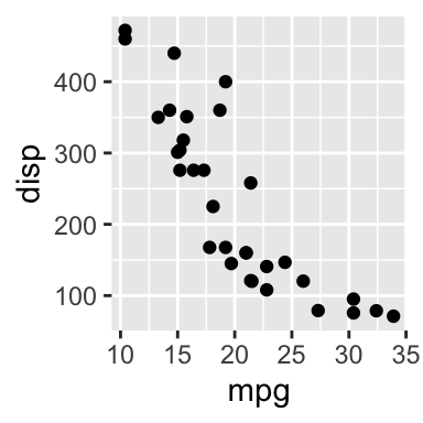

# save each named plot
ggsave(plot = p_scatter, filename = "myscatterplot.png")
ggsave(plot = p_boxplot, filename = "myboxplot.png")

## Warning: Continuous x aesthetic -- did you forget aes(group=...)?

We now have two plots saved. Note that only one plot was printed in the Rmd output because I only called the name of the scatterplot.

across()

I think I need to practice a bit with across() before I really understand it. I’m still kind of digesting when you’d use across() vs just mutating a column at a time, the syntax, etc.

The use of across. I am a little confused with across with where or .fns.

case when and across, I think they just take practice, you explained it well

Yes, across() is difficult! We will use across() in class 5 when we talk about summarize(). I purposefully separated out these two usages because I wanted to introduce it, and then have you see it again once you had time to let it sink in. It will be a while until you will have homework practice with this but I encourage you to try it in your midterm project if you are brave!

Some of the Mutate portion since there are so many applications for Mutate

mutate is still a little blurry for me - but I am sure I will get it with more practice!

There are so many ways to use mutate()! I could probably show 3 hours worth of mutate examples. We will keep using it throughout the class because it’s probably the most useful tidyverse function, honestly.

smoke_new <- smoke_complete %>% mutate( alive = (vital_status == "alive"), alive1 = 1*(vital_status == "alive") ) Not 100% clear what R is doing to create the T/F then 0/1 binary variables.

Let’s break this down in parts, showing what’s happening with just vectors, not a data.frame:

# here is a character vector, a subset of vital_status
myvec <- c("dead","alive", "dead", "alive", "alive")
# R will tell us this is a character vector:
class(myvec)

## [1] "character"

# Now let's run that first code "test" which is a boolean statement using a logical operator ==
myvec == "alive"

## [1] FALSE  TRUE FALSE  TRUE  TRUE

# we see that this gives TRUE, FALSE, TRUE
# this is actually a vector, let's save it as such
myvec_boolean <- myvec == "alive"
myvec_boolean

## [1] FALSE  TRUE FALSE  TRUE  TRUE

# R will tell us this is a logical (= boolean, which means true/false) vector:
class(myvec_boolean)

## [1] "logical"

# now let's multiply it by 1
1*myvec_boolean

## [1] 0 1 0 1 1

# do you see how it turns into 0s and 1s? TRUEs become 1s, FALSEs because 0s
# Let's save it as a vector
myvec_numeric <- 1*myvec_boolean
# now we've turned myvec from a character vector into a binary numeric vector
class(myvec_numeric)

## [1] "numeric"

myvec_numeric

## [1] 0 1 0 1 1

# We could have done this all at once:
1*(myvec=="alive")

## [1] 0 1 0 1 1

booleans. When are they more useful?

Hopefully the example above gives some insight into how they can be useful. I will say as a data type, I don’t use them much, other than to create new variables as above. We also use boolean statements in our filtering and in case_when(), for instance

mtcars %>% filter(cyl==4) # cyl==4 is a TRUE/FALSE value
mtcars %>% select(where(is.numeric)) # is.numeric is TRUE/FALSE
mtcars %>% mutate(
  cyl_cat = case_when(
    cyl < 6 ~ "low", # cyl < 6 is TRUE/FALSE
    cyl >=6 ~ "high" # cyl >= 6 is TRUE/FALSE
  )
)

NA

I’m not sure if this means “not applicable” or, if NA missing values are muddy! I’ll keep trying to go over how we deal with missing data, we’ll see some challenges with NA in class 5.

Bonus muddy point that I’ve noticed confusion on. What is our output from piping code vs what are we saving and why?

Remember that when you manipulate your data, you need to save it as a new data frame (tibble) but be careful about what you are saving.

See these slides for more info.

Clearest points

I love all the examples in this class and I really appreciate that you take time to answer all our questions about syntax and how you would use these functions! R has so much documentation but it can be really dense and hard to understand, at least for non-programmer me. Having questions answered is just priceless!

This time I watched the lecture the day after, while I do enjoy the social aspect of class, I did find it very helpful to pause, go back to my code, rewind if needed, etc.

I like the pairing of these comments because both are excellent points about the benefits of a class like this! It almost seems too luxurious to spend 11 weeks and tuition dollars on a class just about R, especially when there are approximately 12 million resources online teaching the same thing. But when else would we have a chance to do this in our busy lives, outside of school? The community of learners and having someone to bounce questions and ideas off of is indeed priceless. It’s also great to have the course recorded in such a way that it’s accessible after class. If we were having this class in person, that would be a lot more difficult.

Please add more tricks for displaying data (i.e. ncol and other commands) that help with displaying multiple datapoints.

Will do! I want to get through some advanced data wrangling first, but then we will come back to some more ggplot examples.

Thanks for excellent teaching! It’s very useful for me to learn the foundation of R systematically. Is there possible to add some example of actual project data processing in class?

Yes! I have a a couple data sets in mind for this and will try to implement it in the next couple weeks.

ggplot section

assigning levels of a factor and ggplot

ggplots are becoming a lot more clear to me - they confused me last quarter, so thank you !

Great news, I’m so glad!